Lec 08-1 딥러닝의 기본 개념: 시작과 XOR 문제

1. Activation Functions


   사람의 신경을 연구하여 유사 구조로 만듦

2. XOR Problem :


   1) 선형적 논리구조로는 풀지 못함. 

   2) Perceptrons (1969 ) by Marvin Minsky, founder of the MIT AI Lab


   3) Backpropagation (1974, 1982 by Paul Werbos,  1986 by Hinton)


3. Convolutional Neural Networks

   1) 고양이 뇌 실험 

    - 뇌가 이미지를 판단할 때 전체를 사용하는 것이 아니라 그림의 형태에 따라 일부의 뉴런만 사용한다. 

    2) 부분만 사용하여 연산한 후 나중에 합치는 방식 : LeCun 


4. Big Problem


  1) Backpropagation just did not work well for normal neural nets with many

  2) Other rising machine learning algorithms: SVM, RandomForest, etc.

  3) 1995 “Comparison of Learning Algorithms For Handwritten Digit Recognition” by LeCun et al. 

     found that this new approach worked better


Lec 08-2 딥러닝의 기본 개념 2: back-propagation 과 2006/2007 '딥'의 출현

1. Breakthrough : in 2006 and 2007 by Hinton and Bengio

  1) Neural networks with many layers really could be trained well,

     if the weights are initialized in a clever way rather than randomly.

  2) Deep machine learning methods are more efficient for difficult problems than shallow methods.

  3) Rebranding to Deep Nets, Deep Learning


2. ImageNet Classification (2012 ) : 26.2% -> 15.3 %  

   1) 2015년 standford 연구생이 코딩으로 개발한 건보다, CNN을 이용해서 개발한 모델이 정확하게 예측함


Lab 08 Tensor Manipulation
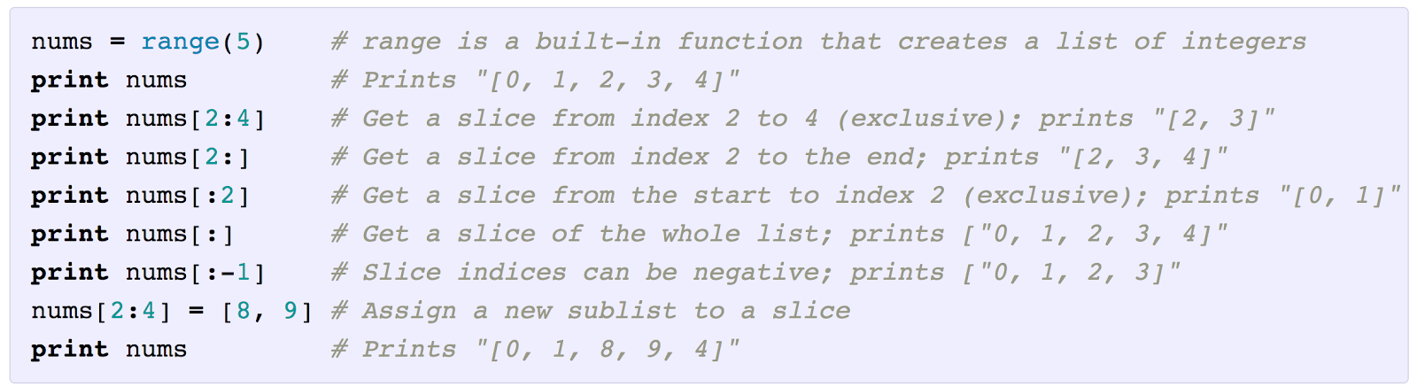
1. Array  

  1) Simple Array [1D]

t = np.array([0., 1., 2., 3., 4., 5., 6.])

pp.pprint(t)

print(t.ndim) # rank

print(t.shape) # shape

print(t[0], t[1], t[-1])

print(t[2:5], t[4:-1])

print(t[:2], t[3:])

array([ 0.,  1.,  2.,  3.,  4.,  5.,  6.])

1   -> 김성훈 교수님 예제 잘못되어 있음 

(7,)

0.0 1.0 6.0

[ 2.  3.  4.] [ 4.  5.]

[ 0.  1.] [ 3.  4.  5.  6.]


  2) 2D Array 

t = np.array([[1., 2., 3.], [4., 5., 6.], [7., 8., 9.], [10., 11., 12.]])

pp.pprint(t)

print(t.ndim) # rank

print(t.shape) # shape

array([[  1.,   2.,   3.],

       [  4.,   5.,   6.],

       [  7.,   8.,   9.],

       [ 10.,  11.,  12.]])

2

(4, 3)


  3) Shape, Rank, Axis

Shape : 배열의 크기  - 가장 안쪽에서 뒤에서 부터 표시

Rank : 배열의 차원

Axis : 배열 요소의 순서 ( X :0 , Y : 1, Z : 3) 


  4) MatMul Vs multiply 

matrix1 = tf.constant([[3., 3.]])

matrix2 = tf.constant([[2.],[2.]])


tf.matmul(matrix1, matrix2).eval()

(matrix1*matrix2).eval()

[[ 12.]]

[[ 6.  6.]

 [ 6.  6.]]


  5) Watch Out Broadcast


2. Function

  1) Reduce mean 

tf.reduce_mean([1, 2], axis=0).eval()

x = [[1., 2.],

     [3., 4.]]

tf.reduce_mean(x).eval()

tf.reduce_mean(x, axis=0).eval()

tf.reduce_mean(x, axis=1).eval()

tf.reduce_mean(x, axis=-1).eval()

1

2.5

[ 2.  3.]

[ 1.5  3.5]

[ 1.5  3.5]


  2) Reduce sum

x = [[1., 2.],

     [3., 4.]]

tf.reduce_sum(x).eval()

tf.reduce_sum(x, axis=0).eval()

tf.reduce_sum(x, axis=-1).eval()

tf.reduce_mean(tf.reduce_sum(x, axis=-1)).eval()

10.0

[ 4.  6.]

[ 3.  7.]

5.0


  3) Argmax : 가장 큰 값의 위치가 어디냐? 

x = [[0, 1, 2],

     [2, 1, 0]]

tf.argmax(x, axis=0).eval()

tf.argmax(x, axis=1).eval()

tf.argmax(x, axis=-1).eval()

[1 0 0]

[2 0]

[2 0]


  4) Reshape, squeeze, expand

t = np.array([[[0, 1, 2], 

               [3, 4, 5]],              

              [[6, 7, 8], 

               [9, 10, 11]]])

t.shape

tf.reshape(t, shape=[-1, 3]).eval()

tf.reshape(t, shape=[-1, 1, 3]).eval()

tf.squeeze([[0], [1], [2]]).eval()

tf.expand_dims([0, 1, 2], 1).eval()

(2, 2, 3)

[[ 0  1  2]

 [ 3  4  5]

 [ 6  7  8]

 [ 9 10 11]]

[[[ 0  1  2]]


 [[ 3  4  5]]


 [[ 6  7  8]]


 [[ 9 10 11]]]

[0 1 2]

[[0]

 [1]

 [2]]


  5) Onehot : 

tf.one_hot([[0], [1], [2], [0]], depth=3).eval()

t = tf.one_hot([[0], [1], [2], [0]], depth=3)

tf.reshape(t, shape=[-1, 3]).eval()

[[[ 1.  0.  0.]]

 [[ 0.  1.  0.]]

 [[ 0.  0.  1.]]

 [[ 1.  0.  0.]]]


[[ 1.  0.  0.]

 [ 0.  1.  0.]

 [ 0.  0.  1.]

 [ 1.  0.  0.]]


  6) Cast / Stack /ones-zeros / zip

tf.cast([1.8, 2.2, 3.3, 4.9], tf.int32).eval()

tf.cast([True, False, 1 == 1, 0 == 1], tf.int32).eval()

#Stack

x = [1, 4]

y = [2, 5]

z = [3, 6]

# Pack along first dim.

tf.stack([x, y, z]).eval()

tf.stack([x, y, z], axis=1).eval()

x = [[0, 1, 2],

     [2, 1, 0]]

tf.ones_like(x).eval()

tf.zeros_like(x).eval()

#Zip

for x, y in zip([1, 2, 3], [4, 5, 6]):

    print(x, y)

for x, y, z in zip([1, 2, 3], [4, 5, 6], [7, 8, 9]):

          print(x, y, z)[1 0 0]

===cast

[1 2 3 4]

[1 0 1 0]

===stack

[[1 4]

 [2 5]

 [3 6]]

[[1 2 3]

 [4 5 6]]

===ones, zeros

[[1 1 1]

 [1 1 1]]

[[0 0 0]

 [0 0 0]]

===zip

1 4

2 5

3 6

1 4 7

2 5 8

3 6 9

Posted by 꿈을펼쳐라
,

Lec 07-1 Learning Rate, Overfitting and Regularization

1. Determining Learning Rate

    1) Try Several learning Rates ( start with 0.01 )

    2) Observe the cost function 

    3) Check it goes down in a reasonable rate 

      - 너무 크면 divergence ,  너무 작은면 늦게 수렴


2. Data(X) Preprocessing for gradient descent 

   1) RAW data가 편중되어 있을 경우, 특정 변수의 민감도가 높거나 낮아질 수 있음. 

   2) Normalization 


    3) Standardization 


           X_std[:,0] = (X[:0] - X[:,0].mean()) / X[:,0].std()   


2. Regularization  

   1) OverFitting 

      - Our model is very good with training data set (with memorization)

      - Not good at test dataset or in real use

    2) Solutions for overfitting 

       - More Training data 

       - Reduce the number of features 

       - Regularization 


    3) Regularization 

       - Let's not have too big numbers in the weight      


        ( Loss함수에 Weight크기를 포함하도록 함으로써 해당 값도 최소화하는 경우를 찾고자 함)  

       - with Tensorflow 

          l2reg = 0.001 * tf.reduce_sum(tf.square(W)) 


Lec 07-2: Training/Testing Data Set


1. Data set 


2. Online Learning 

    1) 데이터 셋을 여러 단위로 분리해서 예측 진행

    2) 이전 단계에서 예측돼었던 내용이 새로운 데이터 셋 예측에서도 동일한 영향을 주여야 함 


3. M NIST Data set


Lab 07-1: training/test dataset, learning rate, normalization


1. Test Dataset  & Learning Rate  

  0) Test Data

   # Evaluation our model using this test dataset

   x_test = [[2, 1, 1],          

            [3, 1, 2],       

            [3, 3, 4]]

   y_test = [[0, 0, 1],

             [0, 0, 1],

             [0, 0, 1]]


   1) optimizer = tf.train.GradientDescentOptimizer(learning_rate=1e-10).minimize(cost)

TOOL Small : Local Min. No Progress


200 5.73203 [[ 0.80269569  0.67861289 -1.21728313]

 [-0.3051686  -0.3032113   1.50825703]

 [ 0.75722361 -0.7008909  -2.10820389]]

Prediction: [0 0 0]

Accuracy:  0.0

   2) optimizer = tf.train.GradientDescentOptimizer(learning_rate=1.5).minimize(cost)

TOOL Large : Divergen


200 nan [[ nan  nan  nan]

 [ nan  nan  nan]

 [ nan  nan  nan]]

Prediction: [0 0 0]

Accuracy:  0.0

  3) optimizer = tf.train.GradientDescentOptimizer(learning_rate=0.1).minimize(cost)

Proper Initial : 


200 0.670909 [[-1.15377057  0.2814692   1.13632655]

 [ 0.37484601  0.18958248  0.33544892]

 [-0.35609847 -0.43973017 -1.256042  ]]

Prediction: [2 2 2]

Accuracy:  1.0


2. Normalized input

  1) Large Value Raw Data 

     y = np.array([[828.659973, 833.450012, 908100, 828.349976, 831.659973],

                   [823.02002, 828.070007, 1828100, 821.655029, 828.070007],

                   [819.929993, 824.400024, 1438100, 818.97998, 824.159973],

                   [816, 820.958984, 1008100, 815.48999, 819.23999],

                   [819.359985, 823, 1188100, 818.469971, 818.97998],

               [819, 823, 1198100, 816, 820.450012],

                   [811.700012, 815.25, 1098100, 809.780029, 813.669983],

                   [809.51001, 816.659973, 1398100, 804.539978, 809.559998]])

100 Cost:  nan 

Prediction:

 [[ nan]

 [ nan]

 [ nan]

 [ nan]

 [ nan]

 [ nan]

 [ nan]

 [ nan]]


Process finished with exit code 0


  2) Normalized input 

def MinMaxScaler(data):

    numerator = data - np.min(data, 0)

    denominator = np.max(data, 0) - np.min(data, 0)

    # noise term prevents the zero division

    return numerator / (denominator + 1e-7)


...


xy = MinMaxScaler(xy)


100 Cost:  0.0136869 

Prediction:

 [[ 1.12295258]

 [ 0.63500863]

 [ 0.53340685]

 [ 0.4315863 ]

 [ 0.53191048]

 [ 0.55868214]

 [ 0.15761785]

 [ 0.14425412]]


Process finished with exit code 0


Lab 07-2: Meet MNIST Dataset


1. MNIST  Image

  1) 28 * 28 * 1 Image (Binary Bitmap


# MNIST data image of shape 28 * 28 = 784

X = tf.placeholder(tf.float32, [None, 784])

# 0 - 9 digits recognition = 10 classes

Y = tf.placeholder(tf.float32, [None, nb_classes])


2. Reading Data and set variables


from tensorflow.examples.tutorials.mnist import input_data

# Check out https://www.tensorflow.org/get_started/mnist/beginners for

# more information about the mnist dataset

mnist = input_data.read_data_sets("MNIST_data/", one_hot=True)


nb_classes = 10


# MNIST data image of shape 28 * 28 = 784

X = tf.placeholder(tf.float32, [None, 784])

# 0 - 9 digits recognition = 10 classes

Y = tf.placeholder(tf.float32, [None, nb_classes])


W = tf.Variable(tf.random_normal([784, nb_classes]))

b = tf.Variable(tf.random_normal([nb_classes]))


...
batch_xs, batch_ys = mnist.train.next_batch(100)
...
print("Accuracy: ", accuracy.eval(session=sess, feed_dict={X: mnist.test.images, Y: mnist.test.labels}))


3. SoftMax

# Hypothesis (using softmax)

hypothesis = tf.nn.softmax(tf.matmul(X, W) + b)


cost = tf.reduce_mean(-tf.reduce_sum(Y * tf.log(hypothesis), axis=1))

optimizer = tf.train.GradientDescentOptimizer(learning_rate=0.1).minimize(cost)


# Test model

is_correct = tf.equal(tf.arg_max(hypothesis, 1), tf.arg_max(Y, 1))

# Calculate accuracy

accuracy = tf.reduce_mean(tf.cast(is_correct, tf.float32))


4. epoch / Batch


1) 데이터가 많을 경우, 모든 데이터를 올리려면 Memory가 많이 필요하므로, Batch로 분할하여 적용

2) epoch [에폭] : 전체 데이터를 한번 모두 훈련하는 과정

3) iteration per epoch = [전체데이터 수] / [batch_size]


# parameters

training_epochs = 15

batch_size = 100


with tf.Session() as sess:

   # Initialize TensorFlow variables

   sess.run(tf.global_variables_initializer())

   # Training cycle

   for epoch in range(training_epochs):

       avg_cost = 0

       total_batch = int(mnist.train.num_examples / batch_size)


       for i in range(total_batch):

           batch_xs, batch_ys = mnist.train.next_batch(batch_size)

           c, _ = sess.run([cost, optimizer], feed_dict={X: batch_xs, Y: batch_ys})

           avg_cost += c / total_batch


       print('Epoch:', '%04d' % (epoch + 1), 'cost =', '{:.9f}'.format(avg_cost))


5. Result


1) 0.8951 정확도


Epoch: 0007 cost = 0.591160339 Epoch: 0008 cost = 0.563868978 Epoch: 0009 cost = 0.541745167 Epoch: 0010 cost = 0.522673571 Epoch: 0011 cost = 0.506782322 Epoch: 0012 cost = 0.492447640 Epoch: 0013 cost = 0.479955830 Epoch: 0014 cost = 0.468893666 Epoch: 0015 cost = 0.458703479 Learning finished Accuracy: 0.8951 Label: [3] Prediction: [5] 


3을 5로 인식한 결과

7을 2로 인식하였다.   아직 89 % 정확도 이니까...


  2) Learning Rate, Epoch 회수 조정으로 정확도를 더 높일 수 있다.  

     Learning Rate = 0.4 ,   Epoch = 100시     92.25%

Epoch: 0098 cost = 0.243552753

Epoch: 0099 cost = 0.243438786

Epoch: 0100 cost = 0.243145558

Learning finished

Accuracy:  0.9225

Label:  [5]

Prediction:  [5]


Posted by 꿈을펼쳐라
,

Lec 06-1 - Softmax Regression 기본 개념 소개

1. Logistic Regression 

    1) Liner Regression의 한계

      -   : 아주 큰수 ,아주 작은 수 적용시에도 선형적 가중치가 적용되어 오차 증가

    2) Logistic Resgression

      - Logistic(Sigmoid) Function : Binary Classification에 적당하도록 아주 큰수, 아주 작은 수 사이에서도 

         0~1 가 되도록 해주는 함수 


2. Multinomial classification

   1)  학점 ABC 구현 - Binary Classification 3개  


Lec 06-2: Softmax classifier 의 cost함수


1. SoftMax Function


   1) Multinomial classification Sigmoid      


     각 Element 가 0 ~ 1 사이값이 되었지만 각각의 상관 관계를 표현하지 못함


   2) SoftMax 


       SCORES                                    POSSIBILITIES


    3) One-Hot Encoding


    4) Cross-entropy cost function 


         S : 예측값,    L : 실제값 


        [check cost function] 


  5) Cross-Entropy vs Logistic Cost  (증명?)  


Lab 06-1: TensorFlow로 Softmax Classification의 구현


1. Hypothesis with SOFTMAX

tf.matmul(X,W) + b 
hypothesis = tf.nn.softmax(tf.matmul(X,W) + b)

2. Cost Function : Cross Entropy

# Cross entropy cost/loss

cost = tf.reduce_mean(-tf.reduce_sum(Y * tf.log(hypothesis), axis=1))


optimizer = tf.train.GradientDescentOptimizer(learning_rate=0.1).minimize(cost)


3. Test & One-Shot Encoding

  1) One Row 

# Testing & One-hot encoding

a = sess.run(hypothesis, feed_dict={X: [[1, 11, 7, 9]]})

print(a, sess.run(tf.arg_max(a, 1)))


raw : [[  1.38904958e-03   9.98601854e-01   9.06129117e-06]]

output : [1]


  2) multi Row 

# Testing & One-hot encoding

all = sess.run(hypothesis, feed_dict={X: [[1, 11, 7, 9], 

                                          [1, 3, 4, 3], 

                                          [1, 1, 0, 1]]})

print(all, sess.run(tf.arg_max(all, 1)))


raw : [[  1.38904958e-03   9.98601854e-01   9.06129117e-06]

[  9.31192040e-01   6.29020557e-02   5.90589503e-03]

[  1.27327668e-08   3.34112905e-04   9.99665856e-01]]

output: [1 0 2]


Lab 06-2: TensorFlow로 Softmax Classification의 구현


1. softmax_cross_entropy_with_logits 


logits = tf.matul(X,W) + b

hypothesis = tf.nn.sotfmax(logits) 


cost = tf.reduce_mean(-tf.reduece_sum(Y * tf.log(hypothesis), axis =1)) 


   cost_i = tf.nn.softmax_coress_entropy_with_logits(logits = logits, labels = Y_one_hot) 


   cost = tf.redue_mean(cost_i)


2. Animal Classification 

  1) load data 

xy = np.loadtxt('data-04-zoo.csv', delimiter= ',', dtype=np.float32) 


x_data = xy[:,0:-1]

y_data = xy[:,[-1]]


hypothesis = tf.nn.sotfmax(logits) 


cost = tf.reduce_mean(-tf.reduece_sum(Y * tf.log(hypothesis), axis =1)) 


  2) ont_hot and reshape 


     Y = tf.placeholder(tf.int32, [None, 1])   # 0~ 6 shape =(?,1)

     Y_one_hot = tf.one_hot(Y, nb_classes)  # one hot shape (?, 1,7) 

     Y_one_hot = tf.reshape(Y_.one_hot, [-1, nb_classes])  # one hot shape (?,7) 


3. Result

'''
Step:     0 Loss: 5.106 Acc: 37.62%
Step:   100 Loss: 0.800 Acc: 79.21%
Step:   200 Loss: 0.486 Acc: 88.12%
Step:   300 Loss: 0.349 Acc: 90.10%
Step:   400 Loss: 0.272 Acc: 94.06%
Step:   500 Loss: 0.222 Acc: 95.05%
Step:   600 Loss: 0.187 Acc: 97.03%
Step:   700 Loss: 0.161 Acc: 97.03%
Step:   800 Loss: 0.140 Acc: 97.03%
Step:   900 Loss: 0.124 Acc: 97.03%
Step:  1000 Loss: 0.111 Acc: 97.03%
Step:  1100 Loss: 0.101 Acc: 99.01%
Step:  1200 Loss: 0.092 Acc: 100.00%
Step:  1300 Loss: 0.084 Acc: 100.00%
...
[True] Prediction: 0 True Y: 0
[True] Prediction: 0 True Y: 0
[True] Prediction: 3 True Y: 3
[True] Prediction: 0 True Y: 0
[True] Prediction: 0 True Y: 0


Posted by 꿈을펼쳐라
,

Lec 05-1 - Logistic Classification의 가설 함수 정의


1. Classification

   - Regression은 특정 값을 예측하는 것에 비해, Classification은 분류 하는 것, 

   - binary Classification은 두개 중 하나 분류,  Ture / False    1/0

   - Spam Detection: Spam or Ham

   - Facebook feed: show or hide

   - Credit Card Fraudulent Transaction detection: legitimate/fraud


2. Logistic Hypothesis

   1) Linear Regression 적용시 문제점 

     - 과도하게 크거나 작은 범위의 값이 적용될 경우 왜곡이 쉽게 발생함   

      EX)  5시간 공부해도 합격, 100 시간 공부해도 합격

   2) 0과 1사이의 Cost Fuction :   logistic function / sigmoid function


       sigmoid  : Curved in two directions, like the letter "S", or the Greek ς (sigma)


                       sigmoid 함수에 대한 이미지 검색결과


    3) Logistic Hypothesis with Vector


Lec 05-2 - Logistic Regression의 cost 함수 설명


1. cost Function   


   1) 기존 코스트 함수 : local minimum 발생으로 최소값을 찾기 곤란함


   2) New Cost Function Concept


    (그래프 그려주는 사이트 : https://www.desmos.com/calculator )


2. understanding New cost Fuction

       - y=1,  H(x) =1     -> correct   -> cost Low  :    C( H(x), y) = -log ( 1 ) = 0 

       - y=1,  H(x) =0     -> wrong    -> cost high  :    C( H(x), y) = -log ( 0 ) = 무한대

       - y=0,  H(x) =0     -> correct   -> cost Low  :    C( H(x), y) = -log ( 1 - 0) = 0 

       - y=0,  H(x) =1     -> wrong    -> cost high :    C( H(x), y) = -log ( 1 - 1) =  - log (0) =  무한대 


3. New cost Fuction  : 두 경우의 선형 조합


4. Minimize Cost


Lab 05: TensorFlow로 Logistic Classification의 구현하기


1. Logistic Regression


2. code


Posted by 꿈을펼쳐라
,

Lab 00 - TensorFlow의 설치 및 기본적인 Operation


1. TensorFlow

  • Open source software library for Numerial computation using data flow graphs.
  • Python

2.  Data Flow Graph

  • Nodes : mathermatical operations
  • Edges : multidimensional data arrays (tensors) communicated between them.

3. Check installation and version    (1.4)


4. Example


  1) Hello world


  2) Node Add 


  3) Placeholder


TensorFlow Mechanics 


1. Build graph using TensorFlow operations

2. feed data and run graph (operation) : sess.run(op)

3. update variables in the grap (and return values)


4. Tenor Ranks, Shapes, and Types

  1) Rank

  2) Shape

  3) Type


Lab 02 - TensorFlow로 구현한 Linear regression


1. Example


2. Linear Regression with Placeholder


Lab 03 - Linear regression : minimize Cost


1. plot cost function


2. Optimized by Hand


3. Optimized by Gradientdecent Function


4. Calculate gradient value


Lab 04 - multi-variable Linear regression


1. Multi-Variable  


2. Multi-Variable with matrix


3. Slice Matrix


4. file data


5. Queue Runners


[에러 발생함]  일단 진행


Posted by 꿈을펼쳐라
,

강의 웹사이트: http://hunkim.github.io/ml/

Facebook: https://www.facebook.com/groups/Tenso...

소스코드: https://github.com/hunkim/DeepLearnin...


Lec 00 - Machine/Deep learning 수업의 개요와 일정


Lec 01 - 머신러닝의 개념과 용어


1. Machine Learning

  - "Field of study that gives computers the ability to learn without being explicitly programmed” Arthur Samuel (1959)


2. Supervised/Unsupervised learning

  - Supervised learning:

     . learning with labeled examples

  - Unsupervised learning: un-labeled data

     . Google news grouping

     . Word clustering


3. Types of supervised learning

  • Predicting final exam score based on time spent

    - regression

  • Pass/non-pass based on time spent

    - binary classification

  • Letter grade (A, B, C, E and F) based on time spent

    - multi-label classification


Lec 02 - Linear Regression의 Hypothesis 와 cost 설명

1. Linear hypothesis

    H(x) = W x + b


2. Cost

    H(x) - y


     H(x) = W x + b


  3. Goal : Minizie Cost


      minimize cost(W,b)


Lec 03 - Linear Regression의 cost 최소화 알고리즘 설명


1. Hypothesis and Cost

  • H(x) = W x


 2. Gradient descent algorithm Minimize cost function

  • formal definition


  • How about Newton-Rapshon algorithm ?


 3. Derivative Calculator : [link]


 4. Check cost function 

  • must be convex curve


Lec 04 - Multi-variable linear regression


1. Hypothesis for multi-variable


2. Hypothesis using Matrix


Posted by 꿈을펼쳐라
,

I. 아나콘다 설치하기


아아콘다 홈페이지 (https://www.anaconda.com/download/)에 접속해서 최신의 아나콘다 버전을 다운받아 설치한다.   (2017/11/26일 현재, Anaconda 5.0.1 버전이 최신)


PATH 환경변수 추가는 이전 설치된 버전보다 먼저 적용되도록하지만, 재설치 및 제거시 문제를 야기시킬 수 있으니 추천하지 않는단다... 일단 빨간색이니 선택하지 않고 진행..


대신에, Anaconda 전용  Prompt 환경에서 시작하는 아이콘이 제공되므로 굳이 Path 추가할 필요가 없단다..


II. TensorFlow 설치


   TensorFlow 홈페이지(https://www.tensorflow.org/install/)에 설치 방법이 자세히 설명되어 있다. 


CPU기반과 GPU기반의 텐서 플로우 설치 방업을 안내해 주고 있는데, 거금을 주고 장만한 1080이니 GPU모드로 설치를 진행해야지...  


하지만, 갑자기 발동된 실험 정신과, 약간의 실수로 다양한 테스트와 실패를 경험하였다.


GPU 기반의  Tensorflow을 설치하기 위해서는 사전에 설치해야할 것이 있다.


1. CUDA Tool Kit 설치 (GPU ) 


      - CUDA Toolkit Download 페이지 : https://developer.nvidia.com/cuda-downloads     

      -  홈페이지에 링크된 최신 버전 9.0을 설치할 경우, dll을 찾지 못하는 에러가 발생함 

      - TensorFlow을 사용하기 위해서는 CUDA Tool Kit 8.0이 설치되어한다.


바로 다운을 진행하면 최신 버전(2017.11.27 현재, 9.0 버전)을 받게되고 이렇게되면 TensorFlow의 현재 버전은 에러가 발생된다. 


이 화면을 보기 싫다면, Tensorflow 소스를 받아서 다시 컴파일 하시던가 (설마요..), 위의 다운로드 페이지 하단에 "Legacy Release" 페이지로 이동한다.


각 버전별로 링크가 되어 있는 이 페이지에서 설치 가이드에서 소개하고 있는 CUDA Toolkit 8.0의 최신 Patch 버전으로 이동한다.


그리고, OS, Version, Installer Type을 선택하고, Base Installer와 Patch2 버전을 각각 다운받아 설치 한다.


CUDA Toolkit 8.0을 설치할 때, 아래와 같은 경고가 나오지만 무시하고 진행.


2. cuDNN v6.1. 설치


      - cuDNN 다운로드 페이지 : https://developer.nvidia.com/rdp/cudnn-download 

      - 계속 다운을 받으려면 NVIDIA Developer 회원가입을 해야 함.

      - 이전에 설치한 CUDA Tool Kit 8.0에 해당하는 6.0 버전을 선택하고


- OS에 해당하는 버전을 선택하여 다운 받는다.


- cuDNN은 zip으로 압축되어 있고, 특정 디렉토리에 압축을 풀고, 해당 파일을 이전에 설치했던 CUDA Toolkit을 설치한 디렉토리에 덮어 쓴다. 


- 내 경우는  "C:\Program Files\NVIDIA GPU Computing Toolkit\CUDA\v8.0"에 덮어썼다.


3. Tensorflow 설치하기


    이제 마지막 단계, Tensorflow를 설치해보자.   

    먼저, 아나콘다를 실행하기 위해서 시작>Ananconda3 (64bit)를 선택하여 실행창을 연다. 


1)  conda 환경을 생성

(여기서 TF는 임의 환경명이고, 3.6은 설치된 python의 버전이다.  가이드에서는 3.5로 되어 있음) 

(C:\ProgramData\Anaconda3) C:\Users\rgba> conda create -n TF python=3.6


2)  TF 환경 활성화


(C:\ProgramData\Anaconda3) C:\Users\rgba> activate TF


3)  tensorflow 설치 


(TF) C:\Users\rgba> pip install --ignore-installed --upgrade tensorflow-gpu


Ⅲ. TensorFlow 설치


실행창에서 python을 실행하고


(TF) C:\Users\rgba> python


아래와 같이 python 스크립트를 작성하고


>>> import tensorflow as tf

>>> hello = tf.constant('Hello, TensorFlow!') 

>>> sess = tf.Session()

>>> print(sess.run(hello)


실행하면 아래와 같은 결과를 확인.. 


Hello, TensorFlow! 


수고 많으셨습니다.~~~~~~


PS.. 이것 저것 해보다 보니 설치버전을 삭제해야할 경우가 있었다.  혹시 그럴 경우 참고..


 pip 설치 패키지 삭제   


pip uninstall [package name]


conda create 삭제  


conda clean --all 
Posted by 꿈을펼쳐라
,

0. XCode 설치하기 

    최근 Mac에서 개발하지 않고, OS Upgrade를 하다보니 Xcode가 설치 되어 있지 않다.

    Mac에서 Qt개발하기 위해서는 필수라고 하니 우선적으로 설치해야 한다. 


1. Qt 최신 버전 다운 받기 :  https://www.qt.io/developers/


2. Qt 설치파일 실행하기 

일단적으로 진행하면 되지만, 끝부분에 아래와 같은 메시지가 여러번 나올 것이다. 

일단 무시하고 설치 마무리를 하자. 

 (최신 Xcode를 설치해도 위와 같은 메시지가 나오지만, 무시하고 진행하자)


3. XCode 권한 세팅 

   터미널 모드에서 아래 명령어를 실행하여 권한 설정을 마무리 하자.

sudo xcode-select -s /Applications/Xcode.app/Contents/Developer 


4. Qt Creator 실행 & Example Loading

(초기 실행화면에서 맘에 드는 예제를 불러오자, 나는 Qt 3D: Planet QML Example을 선택) 


(Configure Project 에서 일단 Desktop만 선택)


(좌측 하단의 빌드 모드를 선택하고 제일 아래 빌드 버튼을 눌러 빌드를 진행하자. 제발 에러가 없기를...) 


5. 결과 화면 확인 


모든 개발 프로젝트의 시작은 환경 구축이 반이라고 하지 않았던가요?  ㅎㅎ   이제 반은 한 겁니다. ^^  

Posted by 꿈을펼쳐라
,

자전거를 타면서 Garmin이나 Strava App.을 이용해서 경로를 저장하고 있다.  

그러나 각  App. 이나 서비스를 이용하면서 아쉬움들이 있다. 


그래서 생각한 것이 이 경로들을 모아보면 어떤 의미있는 데이터가 있지않을까?

개발자의 욕망이 동한다.   그래 취미삼아 해보자. 


그런데, 집에는 구형 맥북프로, 오피스텔에는 windows Desktop 멀티 프랫폼에서 동작하는 App.을 개발해보리라...


하지만, 정보가 깜깜이니 페북의 "생활코딩" 그룹에 문의 드렸더니 다양한 정보들을 페친들이 주신다. 


그내용을 아주 간단히 정리해 보았다.  


MS의 Visual Studio 기반에 익숙한 개발자들에겐 C# 기반으로 Mac-OS뿐 아니라, 모바일 iOS나 안드로이드 App도 개발할 수 있는 Xamarin은 분명 크나큰 매력으로 다가온다. 


Java Script기반의 Electon도 역시 매력적이고 파워풀한 도구이다. 


하지만 나는 보다 근본적이고 Low-Level의 기술, 그리고 확장성등에서 Qt를 선택했다.  


자 시작이다. 


Posted by 꿈을펼쳐라
,

튜닝문제 1

카테고리 없음 2016. 5. 10. 07:33

ROP TABLE 종목별거래상세 PURGE;

CREATE TABLE 종목별거래상세
(
종목코드 VARCHAR2(5) NOT NULL
, 거래번호 NUMBER NOT NULL
, 대량거래유형코드 VARCHAR2(1) NOT NULL
, 거래일자 VARCHAR2(8) NOT NULL
, 시작가격 NUMBER
, 종료가격 NUMBER
, 거래수량 NUMBER
, 회원번호 VARCHAR2(10)
, 계좌번호 VARCHAR2(20)
, 적요 VARCHAR2(1000)
)
PARTITION BY RANGE (거래일자)
(
PARTITION PR_20160501 VALUES LESS THAN ('20160502')
, PARTITION PR_20160502 VALUES LESS THAN ('20160503')
, PARTITION PR_20160503 VALUES LESS THAN ('20160504')
, PARTITION PR_20160504 VALUES LESS THAN ('20160505')
, PARTITION PR_20160505 VALUES LESS THAN ('20160506')
, PARTITION PR_20160506 VALUES LESS THAN ('20160507')
, PARTITION PR_20160507 VALUES LESS THAN ('20160508')
, PARTITION PR_20160508 VALUES LESS THAN ('20160509')
, PARTITION PR_20160509 VALUES LESS THAN ('20160510')
, PARTITION PR_20160510 VALUES LESS THAN ('20160511')
, PARTITION PR_20160511 VALUES LESS THAN ('20160512')
, PARTITION PR_20160512 VALUES LESS THAN ('20160513')
, PARTITION PR_20160513 VALUES LESS THAN ('20160514')
, PARTITION PR_20160514 VALUES LESS THAN ('20160515')
, PARTITION PR_20160515 VALUES LESS THAN ('20160516')
, PARTITION PR_20160516 VALUES LESS THAN ('20160517')
, PARTITION PR_20160517 VALUES LESS THAN ('20160518')
, PARTITION PR_20160518 VALUES LESS THAN ('20160519')
, PARTITION PR_20160519 VALUES LESS THAN ('20160520')
, PARTITION PR_20160520 VALUES LESS THAN ('20160521')
, PARTITION PR_20160521 VALUES LESS THAN ('20160522')
, PARTITION PR_20160522 VALUES LESS THAN ('20160523')
, PARTITION PR_20160523 VALUES LESS THAN ('20160524')
, PARTITION PR_20160524 VALUES LESS THAN ('20160525')
, PARTITION PR_20160525 VALUES LESS THAN ('20160526')
, PARTITION PR_20160526 VALUES LESS THAN ('20160527')
, PARTITION PR_20160527 VALUES LESS THAN ('20160528')
, PARTITION PR_20160528 VALUES LESS THAN ('20160529')
, PARTITION PR_20160529 VALUES LESS THAN ('20160530')
, PARTITION PR_20160530 VALUES LESS THAN ('20160531')
, PARTITION PR_20160531 VALUES LESS THAN ('201606')
, PARTITION PR_99991231 VALUES LESS THAN ( MAXVALUE )
);

DECLARE
l_거래일자 VARCHAR2(8);
BEGIN
FOR i IN 0..2 LOOP

SELECT TO_CHAR(TO_DATE('20160501','YYYYMMDD') + i, 'YYYYMMDD')
INTO l_거래일자
FROM DUAL;

INSERT
INTO 종목별거래상세
SELECT A.종목코드
, B.거래번호
,(CASE WHEN MOD(ROWNUM, 10000) = 0 THEN 'X' ELSE 'A' END) AS 대량거래유형코드
, l_거래일자
, ROWNUM AS 시작가격
, ROWNUM + 1 AS 종료가격
, ROWNUM * 10 AS 거래수량
, LPAD(ROWNUM, 10, '0') AS 회원번호
, LPAD(ROWNUM, 20, '0') AS 계좌번호
, LPAD(ROWNUM, 200, '0') AS 적요
FROM (
SELECT 'A' || LPAD(ROWNUM, 4, '0') AS 종목코드
FROM DUAL
CONNECT BY
LEVEL <= 250
UNION ALL
SELECT 'B' || LPAD(ROWNUM, 4, '0') AS 종목코드
FROM DUAL
CONNECT BY
LEVEL <= 250
) A
,(
SELECT ROWNUM AS 거래번호
FROM DUAL
CONNECT BY
LEVEL <= 1000
) B
ORDER BY
DBMS_RANDOM.RANDOM();

COMMIT;

END LOOP;
END;
/

CREATE UNIQUE INDEX 종목별거래상세_PK ON 종목별거래상세 (종목코드, 거래번호, 대량거래유형코드, 거래일자) LOCAL UNUSABLE;

ALTER INDEX 종목별거래상세_PK REBUILD PARTITION PR_20160501 PARALLEL 2 NOLOGGING;
ALTER INDEX 종목별거래상세_PK REBUILD PARTITION PR_20160502 PARALLEL 2 NOLOGGING;
ALTER INDEX 종목별거래상세_PK REBUILD PARTITION PR_20160503 PARALLEL 2 NOLOGGING;

ALTER INDEX 종목별거래상세_PK NOPARALLEL;


********************************************************************************

▣ 개선 전 SQL

SELECT *
FROM 종목별거래상세 A
WHERE 거래일자 = '20160501'
AND 대량거래유형코드 = 'X'
ORDER BY
거래번호, 종목코드;


50 rows selected.


Execution Plan
----------------------------------------------------------
Plan hash value: 55875824

---------------------------------------------------------------------------------------------------

| Id | Operation | Name | Rows | Bytes | Cost (%CPU)| Time | Pstart| Pstop |

---------------------------------------------------------------------------------------------------

| 0 | SELECT STATEMENT | | 49 | 28665 | 5988 (13)| 00:01:12 | | |

| 1 | SORT ORDER BY | | 49 | 28665 | 5988 (13)| 00:01:12 | | |

| 2 | PARTITION RANGE SINGLE| | 49 | 28665 | 5987 (13)| 00:01:12 | 1 | 1 |

|* 3 | TABLE ACCESS FULL | 종목별거| 49 | 28665 | 5987 (13)| 00:01:12 | 1 | 1 |

---------------------------------------------------------------------------------------------------


Predicate Information (identified by operation id):
---------------------------------------------------

3 - filter("거래일자"='20160501' AND "대량거래유형코드"='X')

Note
-----
- dynamic sampling used for this statement (level=2)


Statistics
----------------------------------------------------------
0 recursive calls
0 db block gets
19242 consistent gets
0 physical reads
0 redo size
14501 bytes sent via SQL*Net to client
553 bytes received via SQL*Net from client
5 SQL*Net roundtrips to/from client
1 sorts (memory)
0 sorts (disk)
50 rows processed

********************************************************************************

▣ 전제 조건
1. 대량거래유형코드 = 'X' 조건에 해당하는 데이터는 극소수임
* 일별 데이터 50만 건 중 수십 건 이하임


▣ 문제
1. 개선 후 SQL을 제시하시오.
* 단, 인덱스 변경 불가

2. 오늘 데이터를 포함하여 과거 1달 이상의 넓은 범위를 액세스하는 SQL을 효율적으로 실행할 수 있는 솔루션을 제시하시오.
* 단, 과거 데이터에는 변경이 발생하지 않음
* 종목별거래상세 테이블 및 인덱스 구조를 변경할 수 없음
* 대신, 다른 오브젝트를 마음대로 추가/변경/삭제할 수 있음

Posted by 꿈을펼쳐라
,